2.1. Activation Functions

What is Activation Function?

It’s just a function that you use to get the output of a node.

Why we use Activation functions with Neural Networks?

Activation functions play an integral role in neural networks by introducing nonlinearity. This nonlinearity allows neural networks to develop complex representations and functions based on the inputs that would not be possible with a simple linear regression model (although we have linear activation functions as well).

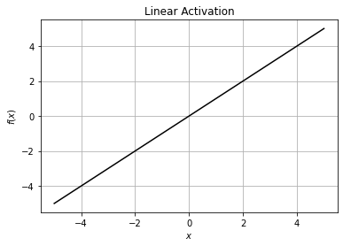
1. Linear

The linear activation function, also known as “no activation,” or “identity function”. This function simply returns its input.

Mathematically it can be represented as:

\[ f(x) = x \]

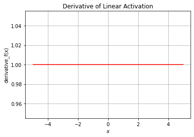
and has derivative

\[ \frac{\partial f(x)}{\partial x} = 1 \]

The linear activation function is often used before the last layer in a neural network for regression. Rather than constraining the fitted values to be in some range or setting half of them equal to 0, we want to leave them as they are.

Consider a dataset (\(x\) value) with \(1000\) samples in range -5 to 5.

x = np.linspace(-5,5,1000)

The linear(x) function below implements the linear activation function whereas the d_linear(x) function implements its derivative (vectorized code instead of using loops)

def linear(x):
    return x

def d_linear(x):
    return np.ones(x.shape)

We can demonstrate both these functions on our dataset (\(x\)) above.

The complete example is listed below.

import numpy as np
import matplotlib.pyplot as plt

def linear(x):
    return x

def d_linear(x):
    return np.ones(x.shape)

x = np.linspace(-5,5,1000)
f = linear(x)
df = d_linear(x)

plt.plot(x, f, 'k')
plt.xlabel("$x$")
plt.ylabel("$f(x)$")
plt.title("Linear Activation")
plt.grid()
plt.show()

plt.plot(x, df, 'r')
plt.xlabel("$x$")
plt.ylabel("derivative_f(x)")
plt.title("Derivative of Linear Activation")
plt.grid()
plt.show()

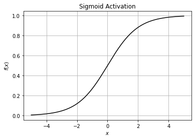
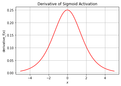
2. Sigmoid

The Sigmoid function (or Logistic Activation function) curve looks like a S-shape. The main reason we use this function is that it takes any real value as input and outputs values in the range of 0 to 1.

The larger the input (more positive), the closer the output value will be to 1.0, whereas the smaller the input (more negative), the closer the output will be to 0.0

Mathematically it can be represented as:

\[f(x) = \frac{1}{1+e^{-x}}\]

Now, a convenient fact about the sigmoid function is that we can express its derivative in terms of itself.

\[\frac{\partial f(x)}{\partial x} = \frac{e^{-x}}{\left( 1 + e^{-x} \right)^2} = \frac{1}{1 + e^{-x}} \cdot \frac{e^{-x}}{1 + e^{-x}} = f(x)\left(1 - f(x)\right)\]

The sigmoid(x) function below implements the sigmoid activation function whereas the d_sigmoid(x) function implements its derivative (vectorized code instead of using loops)

def sigmoid(x):
    '''
    Parameters
    
    x: input matrix of shape (m, d) 
    where 'm' is the number of samples (or rows)
    and 'd' is the number of features (or columns)
    '''
    return 1/(1+np.exp(-x))

def d_sigmoid(x):
    return sigmoid(x) * (1-sigmoid(x))

We can demonstrate both these functions on our dataset (\(x\)) used above.

The complete example is listed below.

import numpy as np
import matplotlib.pyplot as plt

def sigmoid(x):
    '''
    Parameters
    
    x: input matrix of shape (m, d) 
    where 'm' is the number of samples (or rows)
    and 'd' is the number of features (or columns)
    '''
    return 1/(1+np.exp(-x))

def d_sigmoid(x):
    return sigmoid(x) * (1-sigmoid(x))

x = np.linspace(-5,5,1000)
f = sigmoid(x)
df = d_sigmoid(x)

plt.plot(x, f, 'k')
plt.xlabel("$x$")
plt.ylabel("$f(x)$")
plt.title("Sigmoid Activation")
plt.grid()
plt.show()

plt.plot(x, df, 'r')
plt.xlabel("$x$")
plt.ylabel("derivative_f(x)")
plt.title("Derivative of Sigmoid Activation")
plt.grid()
plt.show()

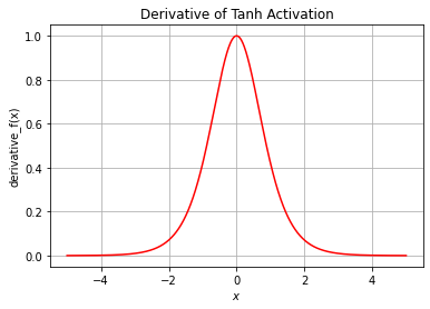
3. Tanh

Tanh is also similar to logistic sigmoid but better because it outputs the value of any real input in the range of -1 to 1 instead of 0 to 1.

Therefore the negative inputs will be mapped strongly negative (near to -1) and the zero inputs will be mapped near zero using tanh activation.

Mathematically it can be represented as:

\[ f(x) = \frac{e^{x}-e^{-x}}{e^{x}+e^{-x}} \]

Again, a convenient fact about the tanh function is that we can express its derivative in terms of itself (we have left the proof as an exercise for the readers).

\[ \frac{\partial f(x)}{\partial x} = 1-f^2(x). \]

The tanh(x) function below implements the tanh activation function whereas the d_tanh(x) function implements its derivative (vectorized code instead of using loops)

def tanh(x):
    '''
    Parameters
    
    x: input matrix of shape (m, d) 
    where 'm' is the number of samples (or rows)
    and 'd' is the number of features (or columns)
    '''
    return (np.exp(x) - np.exp(-x)) / (np.exp(x) + np.exp(-x))

def d_tanh(x):
    return 1-(tanh(x))**2

We can demonstrate both these functions on our dataset (\(x\)) used above.

The complete example is listed below.

import numpy as np
import matplotlib.pyplot as plt

def tanh(x):
    '''
    Parameters
    
    x: input matrix of shape (m, d) 
    where 'm' is the number of samples (or rows)
    and 'd' is the number of features (or columns)
    '''
    return (np.exp(x) - np.exp(-x)) / (np.exp(x) + np.exp(-x))

def d_tanh(x):
    return 1-(tanh(x))**2

x = np.linspace(-5,5,1000)
f = tanh(x)
df = d_tanh(x)

plt.plot(x, f, 'k')
plt.xlabel("$x$")
plt.ylabel("$f(x)$")
plt.title("Tanh Activation")
plt.grid()
plt.show()

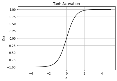
Notice how the values goes from -1 to 1 instead of 0 to 1

plt.plot(x, df, 'r')
plt.xlabel("$x$")
plt.ylabel("derivative_f(x)")
plt.title("Derivative of Tanh Activation")
plt.grid()
plt.show()

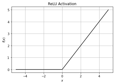
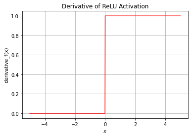
4. ReLU

ReLU is a simple yet extremely common activation function. It stands for Rectified Linear Unit.

Mathematically it can be represented as:

\[ f(x) = \text{max}(x, 0) \]

and has derivative

\[\begin{split} \frac{\partial f(x)}{\partial x} = \begin{cases} 1, & x > 0 \\ 0, & x \leq 0. \end{cases} \end{split}\]

Note: This derivative is not technically defined at 0. In practice, it is very unlikely that we will be applying an activation function to 0 exactly, though in that case the convention is to set its derivative equal to 0.

The ReLU(x) function below implements the ReLU activation function whereas the d_ReLU(x) function implements its derivative (vectorized code instead of using loops)

def ReLU(x):
    '''
    Parameters
    
    x: input matrix of shape (m, d) 
    where 'm' is the number of samples (or rows)
    and 'd' is the number of features (or columns)
    '''
    return x * (x > 0)

def d_ReLU(x):
    return (x>0)*np.ones(x.shape)

We can demonstrate both these functions on our dataset (\(x\)) used above.

The complete example is listed below.

import numpy as np
import matplotlib.pyplot as plt

def ReLU(x):
    '''
    Parameters
    
    x: input matrix of shape (m, d) 
    where 'm' is the number of samples (or rows)
    and 'd' is the number of features (or columns)
    '''
    return x * (x > 0)

def d_ReLU(x):
    return (x>0)*np.ones(x.shape)

x = np.linspace(-5,5,1000)
f = ReLU(x)
df = d_ReLU(x)

plt.plot(x, f, 'k')
plt.xlabel("$x$")
plt.ylabel("$f(x)$")
plt.title("ReLU Activation")
plt.grid()
plt.show()

plt.plot(x, df, 'r')
plt.xlabel("$x$")
plt.ylabel("derivative_f(x)")
plt.title("Derivative of ReLU Activation")
plt.grid()
plt.show()

The ReLU function is far more computationally efficient when compared to the sigmoid and tanh functions.

Only one disadvantage of ReLU is that all the negative input values become zero immediately, which decreases the model’s ability to learn from the data properly (also known as dying ReLU problem).

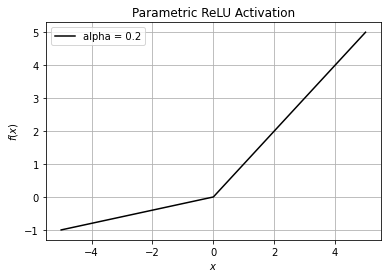
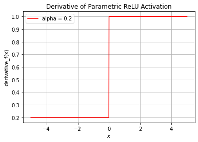
5. Parametric ReLU

It is an attempt to solve the dying ReLU problem as it has a small positive slope \(\alpha\) in the \(x < 0\) area.

Mathematically it can be represented as:

\[\begin{split} f(x) = \begin{cases} x, & x > 0 \\ \alpha x, & x \leq 0. \end{cases} \end{split}\]

and has derivative

\[\begin{split} \frac{\partial f(x)}{\partial x} = \begin{cases} 1, & x > 0 \\ \alpha, & x \leq 0. \end{cases} \end{split}\]

Note: Neural network figures out the slope parameter \(\alpha\) value itself while learning. If this \(\alpha\) is a fixed value (say 0.01), then the activation is called Leaky ReLU.

The PReLU(x, alpha) function below implements the Parametric ReLU activation function (alpha variable or \(\alpha\) is the slope parameter discussed above) whereas the d_PReLU(x, alpha) function implements its derivative (vectorized code instead of using loops)

def PReLU(x, alpha=0.01):
    '''
    Parameters
    alpha: slope parameter (𝛼)

    x: input matrix of shape (m, d) 
    where 'm' is the number of samples (or rows)
    and 'd' is the number of features (or columns)
    '''
    return np.where(x > 0, x, alpha*x) 

def d_PReLU(x, alpha=0.01):
    return np.where(x > 0, 1, alpha) 

We can demonstrate both these functions on our dataset (\(x\)) used above. We will be using the value of \(\alpha = 0.2\)

The complete example is listed below.

import numpy as np
import matplotlib.pyplot as plt

def PReLU(x, alpha=0.01):
    '''
    Parameters
    alpha: slope parameter (𝛼)

    x: input matrix of shape (m, d) 
    where 'm' is the number of samples (or rows)
    and 'd' is the number of features (or columns)
    '''
    return np.where(x > 0, x, alpha*x) 

def d_PReLU(x, alpha=0.01):
    return np.where(x > 0, 1, alpha) 

x = np.linspace(-5,5,1000)
alpha = 0.2
f = PReLU(x, alpha=alpha)
df = d_PReLU(x, alpha=alpha)

plt.plot(x, f, color='k', label="alpha = " + str(alpha))
plt.xlabel("$x$")
plt.ylabel("$f(x)$")
plt.title("Parametric ReLU Activation")
plt.legend()
plt.grid()
plt.show()

plt.plot(x, df, color='r', label="alpha = " + str(alpha))
plt.xlabel("$x$")
plt.ylabel("derivative_f(x)")
plt.title("Derivative of Parametric ReLU Activation")
plt.legend()
plt.grid()
plt.show()

6. Softmax

Note: This activation function is presented only for the sake of completeness. If you are not able to digest it for now, do not worry as we will again be dealing with it in the later part of this course. You can skip it for now!

The Softmax activation function normalizes an input value into a vector of values that follows a probability distribution whose total sums up to 1. The output values are between the range \([0,1]\) which is nice because we are able to avoid binary classification and accommodate as many classes or dimensions in our neural network model.

If the softmax function is used for multi-classification model it returns the probabilities of each class and the target class will have the highest probability.

Mathematically it can be represented as:

\[ f(x_i) = p_i = \frac{e^{x_i}}{\sum_{k=1}^N e^{x_k}} \]

where \(N\) is the total number of samples in \(x\) and \(x_i\) is the \(i^{th}\) sample of \(x\).

It has the following derivative (we have left the proof as an exercise for the readers):

\[\begin{split} \frac{\partial f(x_i)}{\partial x_j} = \frac{\partial p_i}{\partial x_j} = \begin{cases}p_i(1-p_j) & if & i=j \\ -p_j.p_i & if & i \neq j \end{cases} \end{split}\]

or using Kronecker delta:

\[\begin{split} \delta{ij} = \begin{cases} 1 & if & i=j \\ 0 & if & i\neq j \end{cases} \end{split}\]

we can re-write the derivative as:

\[ \frac{\partial p_i}{\partial x_j} = p_i(\delta_{ij}-p_j) \]

To make our softmax function numerically stable, we simply normalize the values in the vector, by multiplying the numerator and denominator with a constant \(C\).

\[\begin{split} \begin{align} p_i &= \frac{e^{x_i}}{\sum_{k=1}^N e^{x_k}} \\ &= \frac{Ce^{x_i}}{C\sum_{k=1}^N e^{x_k}} \\ &= \frac{e^{x_i + \log(C)}}{\sum_{k=1}^N e^{x_k + \log(C)}} \\ \end{align} \end{split}\]

We can choose an arbitrary value for \(\log(C)\) term, but generally \(\log(C)=−\max(x)\) is chosen, as it shifts all of elements in the vector to negative to zero, and negatives with large exponents saturate to zero rather than the infinity, avoiding overflowing and resulting in nan.

The softmax(x) function below implements the numerically stable softmax activation function whereas the d_softmax(x) function implements its derivative (vectorized code instead of using loops)

def softmax(x):
    '''
    Parameters
    x: input matrix of shape (m, d) 
    where 'm' is the number of samples (or rows)
    and 'd' is the number of features (or columns)
    '''
    z = np.array(x) - np.max(x, axis=-1, keepdims=True)
    numerator = np.exp(z)
    denominator = np.sum(numerator, axis=-1, keepdims=True)
    return numerator / denominator

def d_softmax(x):
    x = np.array(x)
    m, d = x.shape
    a = softmax(x)
    tensor1 = np.einsum('ij,ik->ijk', a, a)
    tensor2 = np.einsum('ij,jk->ijk', a, np.eye(d, d))
    return tensor2 - tensor1

We can demonstrate both these functions on the given dataset (\(x\)):

x = [2, 3, 5, 6]

The complete example is listed below.

import numpy as np

def softmax(x):
    '''
    Parameters
    x: input matrix of shape (m, d) 
    where 'm' is the number of samples (or rows)
    and 'd' is the number of features (or columns)
    '''
    z = np.array(x) - np.max(x, axis=-1, keepdims=True)
    numerator = np.exp(z)
    denominator = np.sum(numerator, axis=-1, keepdims=True)
    return numerator / denominator

def d_softmax(x):
    if len(x.shape)==1:
        x = np.array(x).reshape(1,-1)
    else:
        x = np.array(x)
    m, d = x.shape
    a = softmax(x)
    tensor1 = np.einsum('ij,ik->ijk', a, a)
    tensor2 = np.einsum('ij,jk->ijk', a, np.eye(d, d))
    return tensor2 - tensor1

x = np.array([2, 3, 5, 6])
f = softmax(x)
df = d_softmax(x)

print("x =", x)
print("\nSoftmax function output =", f)
print("\nSum of Softmax function =", np.sum(f))
print("\nDerivative of Softmax function output:\n\n", df)

x = [2 3 5 6]

Softmax function output = [0.01275478 0.03467109 0.25618664 0.69638749]

Sum of Softmax function = 1.0

Derivative of Softmax function output:

 [[[ 0.0125921  -0.00044222 -0.0032676  -0.00888227]
  [-0.00044222  0.03346901 -0.00888227 -0.02414451]
  [-0.0032676  -0.00888227  0.19055505 -0.17840517]
  [-0.00888227 -0.02414451 -0.17840517  0.21143195]]]

If we observe the function output for the input value \(6\) we are getting the highest probability. This is what we can expect from the softmax function. Later in classification task, we can use the highest probability value for predicting the target class for the given input features.

Activation class

Lastly, we will be clubbing all of these functions together in a python class Activation.

This class constructor init has the following parameter: activation_type (which is the type of activation we want, default=’sigmoid’)

This class also has a getter function for both (activation and its derivative) as get_activation(x) and get_d_activation(x) respectively

We will be calling the same to calculate the activation of the input \(x\)

import numpy as np

class Activation:

    def __init__(self, activation_type='sigmoid'):
        '''
        Parameters
        
        activation_type: type of activation
        available options are 'sigmoid', 'linear', 'tanh', 'softmax', 'prelu' and 'relu'
        '''
        self.activation_type = activation_type

    def linear(self, x):
        return x

    def d_linear(self, x):
        return np.ones(x.shape)

    def sigmoid(self, x):
        '''
        Parameters
        
        x: input matrix of shape (m, d) 
        where 'm' is the number of samples (in case of batch gradient descent of size m)
        and 'd' is the number of features
        '''
        return 1/(1+np.exp(-x))

    def d_sigmoid(self, x):
        return self.sigmoid(x) * (1-self.sigmoid(x))

    def tanh(self, x):
        return (np.exp(x) - np.exp(-x)) / (np.exp(x) + np.exp(-x))

    def d_tanh(self, x):
        return 1-(self.tanh(x))**2

    def ReLU(self, x):
        return x * (x > 0)

    def d_ReLU(self, x):
        return (x>0)*np.ones(x.shape)

    def PReLU(self, x, alpha=0.2):
        '''
        Parameters
        alpha: slope parameter (𝛼)

        x: input matrix of shape (m, d) 
        where 'm' is the number of samples (or rows)
        and 'd' is the number of features (or columns)
        '''
        return np.where(x > 0, x, alpha*x) 

    def d_PReLU(self, x, alpha=0.2):
        return np.where(x > 0, 1, alpha) 

    def softmax(self, x):
        z = x - np.max(x, axis=-1, keepdims=True)
        numerator = np.exp(z)
        denominator = np.sum(numerator, axis=-1, keepdims=True)
        softmax = numerator / denominator
        return softmax

    def d_softmax(self, x):
        if len(x.shape)==1:
            x = np.array(x).reshape(1,-1)
        else:
            x = np.array(x)
        m, d = x.shape
        a = self.softmax(x)
        tensor1 = np.einsum('ij,ik->ijk', a, a)
        tensor2 = np.einsum('ij,jk->ijk', a, np.eye(d, d))
        return tensor2 - tensor1

    def get_activation(self, x):
        if self.activation_type == 'sigmoid':
            return self.sigmoid(x)
        elif self.activation_type == 'tanh':
            return self.tanh(x)
        elif self.activation_type == 'relu':
            return self.ReLU(x)
        elif self.activation_type == 'linear':
            return self.linear(x)
        elif self.activation_type == 'prelu':
            return self.PReLU(x)
        elif self.activation_type == 'softmax':
            return self.softmax(x)
        else:
            raise ValueError("Valid Activations are only 'sigmoid', 'linear', 'tanh' 'softmax', 'prelu' and 'relu'")

    def get_d_activation(self, x):
        if self.activation_type == 'sigmoid':
            return self.d_sigmoid(x)
        elif self.activation_type == 'tanh':
            return self.d_tanh(x)
        elif self.activation_type == 'relu':
            return self.d_ReLU(x)
        elif self.activation_type == 'linear':
            return self.d_linear(x)
        elif self.activation_type == 'prelu':
            return self.d_PReLU(x)
        elif self.activation_type == 'softmax':
            return self.d_softmax(x)
        else:
            raise ValueError("Valid Activations are only 'sigmoid', 'linear', 'tanh', 'softmax', 'prelu' and 'relu'")

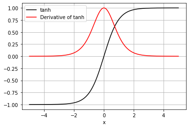
Validating our Activation class

we will use activation_type=’tanh’ and plot the tanh and its dervative on the same graph

import matplotlib.pyplot as plt
import numpy as np

# available options are 'sigmoid', 'linear', 'tanh', 'softmax', 'prelu' and 'relu'
activation_type = 'tanh'

# defining a class object
activation = Activation(activation_type=activation_type)

# x values
x = np.linspace(-5,5,1000)

# calling getter method to get the activation function value (and its derivative)
f = activation.get_activation(x)
df = activation.get_d_activation(x)

# Plotting
plt.plot(x, f, label=activation_type, color='k')
plt.plot(x, df, label='Derivative of ' + activation_type, color='r')
plt.legend()
plt.xlabel('x')
plt.grid()
plt.show()