2.13. Shortcut to calculate forward pass and backpropagation across layers
Contents
2.13. Shortcut to calculate forward pass and backpropagation across layers#
Since we have only five different operations (mentioned below; from whatever we have learned till now) that can performed on the input (\(X\)) to get a certain output (\(Z\)), so, the following rule can help us evaluate the forward pass and backpropagation error through that particular operation. This is same as obtaining forward pass and backpropagation through the computational graphs. Let me explain.
Note: \(Q^T\) denotes the transpose of the matrix \(Q\) and \(\sum_c\) denotes sum along the columns (i.e. sum of column-1 then sum of column-2 and so on) to get a vector of length same as number of columns.
1. Matrix Multiplication \((*)\)
Let \((*)\) denote the matrix multiplication between Input \(X\) of size \((m,d)\) and the parameter of this blackbox (Matrix Multiplication operation) \(W\) of size \((d,h)\) and let the Output be \(Z\), whose size will be \((m,h)\).
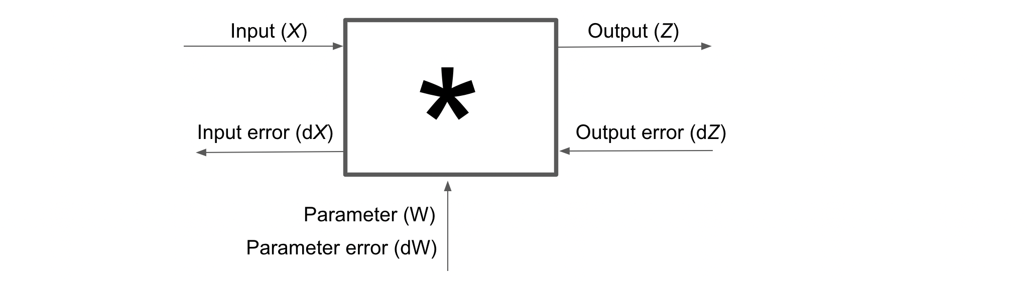
Forward Propagation
Backpropagation
Output
\[dX_{(m,d)} = dZ_{(m,h)} * W^T_{(h,d)}\]Parameter
\[dW_{(d,h)} = X^T_{(d,m)} * dZ_{(m,h)}\]
2. Addition \((+)\)
Let \((+)\) denote addition between Input \(X\) of size \((m,d)\) and the parameter of this blackbox, \(b\) of size \((d,1)\) and let the Output be \(Z\), whose size will be \((m,d)\).

Forward Propagation
Backpropagation
Output
\[dX = dZ\]Parameter
\[db = \sum_c dZ\]
3. Activation \(f(.)\)
Let \(f(.)\) be the activation function that transforms Input \(X\) of size \((m,d)\) to an Output \(Z\) of same size as that of \(X\). Since, the operation is performed element wise on \(X\) (each element of \(X\) got transformed into the respective elements of \(Z\) through \(f(.)\)), so let us denote \(\odot\) as an element wise multiplication operation. This black box has no parameters.
Note: \(f'(.)\) denotes the derivative of the activation function. We have already explained how to calculate these derivatives here (link to previous chapter)

Forward Propagation
Backpropagation
Output
\[dX = dZ \odot f'(X)\]Parameter
\[\text{None}\]
4. Dropout \((\text{DR})\)
Let \(\text{DR}\) denote the dropout operation on Input \(X\) of size \((m,d)\) to get an Output \(Z\) of same size as that of \(X\). We have already calculated the forward (\(Z\)) and back propagation (\(dX\)) results for dropout here (link to previous chapter).

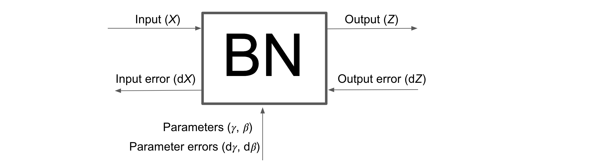
4. Batch Normalization \((\text{BN})\)
Let \(\text{BN}\) denote the Batch Normalization operation on Input \(X\) of size \((m,d)\) to get an Output \(Z\) of same size as that of \(X\). We have already calculated the forward (\(Z\)) and back propagation (\(dX\)) results for Batch Normalization here (link to previous chapter).
Example#
Consider the network shown below (assume that the hidden layer also contains activation function)
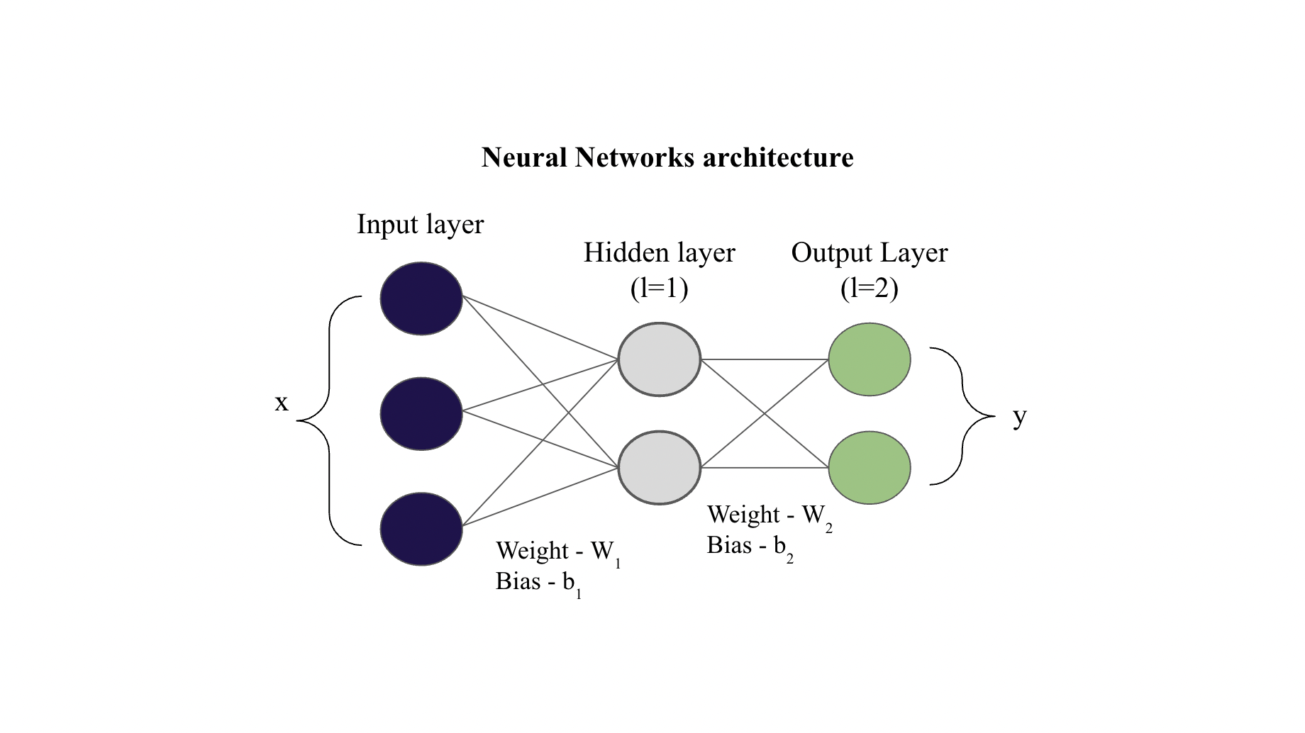
Following the different operations discussed above, we can break this network into series of operations as shown below.
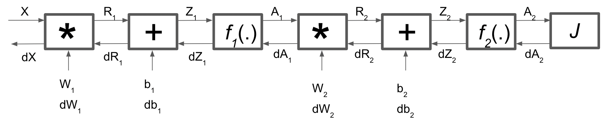
Forward Propagation
After this we calculate our cost function \(J(W, b)\) and then we perform backpropagation.
Backpropagation
\(dA_2\) can be calculated based on the type of cost function we are using. For example if the cost function is MSE, then \(dA_2 = A_2-y\) (where \(y\) is the target variable).
Didn’t know Backpropagation can be so easy and intuitive