4.1. Traditional Word Embeddings
Contents
4.1. Traditional Word Embeddings#
Word Embedding in simple term is a representation of a word. Word embedding techniques are used for analysing texts. It is capable of capturing context of a word in a document, semantic and syntactic similarity, relation with other words, etc.
But why do we need it? The problem with Machine Learning or Deep Learning models is that it can’t understand texts. So, we have to convert the words into numbers.
Thus, loosely speaking, word embedding are vector representations of a particular word. It allows words with similar meaning to have a similar representation. They can also approximate meanings.
So, how do they capture the context? We will get to it soon. But in this section we will be describing various ways to find the vector representation of a word using the Traditional Word Embeddings approach.
One-Hot Vectors#
You can follow this write-up (link to previous chapter) to know about One Hot Encoding.
Let us consider an example, where we are provided with the following sentence:
Sentence: We are learning word embeddings.
If we construct an exhaustive vocabulary from this sentence (let’s call it \(V\)), it would have
V = {We, are, learning, word, embeddings}
If we construct one hot encoded vector for each of these words in V, then
Here, every word has been assigned a unique vector and the length of our one-hot encoded vector would be equal to the size of \(V\) \((|V|=5)\).
Note
In one hot encoding representations, all the words are independent of each other, and therefore there is no relationship between words.
One hot encoding is computionally expensive because in reality the vocabulary size could be billions if not trillions and thus such representation is not feasible in real life scenario.
Defining Corpus#
Let us assume, our corpus (meaning collection of written texts) comprises of 4 documents (here documents means sentences).
Corpus
This is the first document. This document is the second document. This is the third one. Is this the first document?
Document-1 (Sentence-1): This is the first document.
Document-2 (Sentence-2): This document is the second document.
Document-3 (Sentence-3): This is the third one.
Document-4 (Sentence-4): Is this the first document?
Now assume that we have removed all the punctuations from the documents and also we have converted all the words to lower case. This is what pre-processed documents would look like:
Document-1 (Sentence-1): this is the first document
Document-2 (Sentence-2): this document is the second document
Document-3 (Sentence-3): this is the third one
Document-4 (Sentence-4): is this the first document
Now, if we construct an exhaustive vocabulary from this pre-processed corpus (let’s call it \(V\)), it would have
V = {'document', 'this', 'one', 'first', 'second', 'third', 'is', 'the'}
Count-Vector or Bag-of-Words (BOW)#
It is one of the simplest ways of doing text vectorization. It creates a document term matrix, that indicates if a particular word (or a token or a term) appears in the document. Each element (number) of this matrix represents the frequency of the word in that particular document.
document |
this |
one |
first |
second |
third |
is |
the |
|
|---|---|---|---|---|---|---|---|---|
Document-1 |
1 |
1 |
0 |
1 |
0 |
0 |
1 |
1 |
Document-2 |
2 |
1 |
0 |
0 |
1 |
0 |
1 |
1 |
Document-3 |
0 |
1 |
1 |
0 |
0 |
1 |
1 |
1 |
Document-4 |
1 |
1 |
0 |
1 |
0 |
0 |
1 |
1 |
Now, a column in the above matrix can also be understood as a word vector representation for the corresponding word.
For Example,
Vector for document is [1, 2, 0, 1],
Vector for first is [1, 0, 0, 1], and so on.
Hence we see that even though the length of the vocabulary \(|V|=8\), still the vector size for each word turns out to be of length-4. This way we have converted the words into numbers.
Since the calculation is just based on count and there is no consideration for the context of a word, the method proves to be less beneficial.
Co-occurrence Matrix#
The co-occurrence matrix indicates how many times the row word (e.g. ‘is’ from the above corpus mentioned in Defining Corpus section) is surrounded (in a sentence, or in the \(±2\) sized word window which can vary depending on the application type) by the column word (e.g. ‘the’).
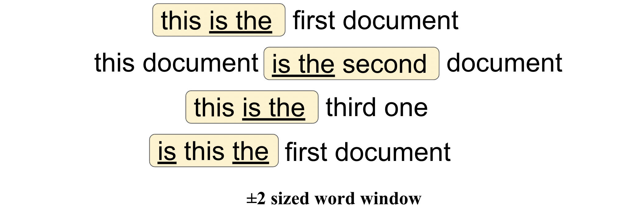
The entry ‘4’ in the following table (which is the co-occurrence matrix), means that we had 4 sentences in our text where is was surrounded by the.
document |
first |
is |
one |
second |
the |
third |
this |
|
|---|---|---|---|---|---|---|---|---|
document |
0 |
2 |
1 |
0 |
1 |
4 |
0 |
1 |
first |
2 |
0 |
1 |
0 |
0 |
2 |
0 |
1 |
is |
1 |
1 |
0 |
0 |
1 |
4 |
1 |
4 |
one |
0 |
0 |
0 |
0 |
0 |
1 |
1 |
0 |
second |
1 |
0 |
1 |
0 |
0 |
1 |
0 |
0 |
the |
4 |
2 |
4 |
1 |
1 |
0 |
1 |
3 |
third |
0 |
0 |
1 |
1 |
0 |
1 |
0 |
0 |
this |
1 |
1 |
4 |
0 |
0 |
3 |
0 |
0 |
Note that the co-occurrence matrix is always symmetric - the entry with the row word ‘the’ and the column word ‘is’ will be 4 as well (as these words co-occur in the very same sentences).
N-Gram#
Similar to the count vectorization technique, in the N-Gram method, a document term matrix is generated and each cell represents the count (frequency of the term in the document).
The difference in the N-grams method is that the count represents the combination of adjacent words of length \(n\) in the document.
Note
Count vectorization is N-Gram where n=1.
For example, just consider only the document-1 (from above example) for now.
Document-1: this is the first document
Unigrams (n=1)
If \(n=1\), i.e unigrams, the word pairs would be ["this", "is", "the", "first", "document"] as we would expect in case of count vector (Bag-of-Words).
Bigrams (n=2)
If \(n=2\), i.e bigrams, the word pairs would be ["this is", "is the", "the first", "first document"]
Trigrams (n=3)

If \(n=3\), i.e trigrams, the word pairs would be ["this is the", "is the first", "the first document"]
Unlike BOW, it maintains word order but there are too many features and therefore it is computationally expensive. Also, choosing the optimal value of “\(n\)” is not that easy task.
TF-IDF (with code from scratch)#
TF-IDF stands for Term Frequency-Inverse Document Frequency. It is a statistical measure that evaluates how relevant a word is to a document in a collection of documents.
This method is an improvement over the Count Vector method as the frequency of a particular word is considered across the whole corpus and not just a single document.
The main idea is to give more weight to the words which are very specific to certain documents whereas to give less weight to the words which are more general and occur across most documents.
For example, if we look at the term document matrix formed in the Count Vector section,
document |
this |
one |
first |
second |
third |
is |
the |
|
|---|---|---|---|---|---|---|---|---|
Document-1 |
1 |
1 |
0 |
1 |
0 |
0 |
1 |
1 |
Document-2 |
2 |
1 |
0 |
0 |
1 |
0 |
1 |
1 |
Document-3 |
0 |
1 |
1 |
0 |
0 |
1 |
1 |
1 |
Document-4 |
1 |
1 |
0 |
1 |
0 |
0 |
1 |
1 |
just look at the words {"this", "is", "the"}, they occur in all the documents and therefore they are less relevant in finding context of the word in a particular document. If you say word "this" then it is difficult to figure out which document you are referring to whereas if you say "one", then it is obvious that you are referring to document-3!
Let us see how to calculate this TF-IDF for given collection of documents (consider the same example as in Count-Vector section).
Document-1 (Sentence-1): this is the first document
Document-2 (Sentence-2): this document is the second document
Document-3 (Sentence-3): this is the third one
Document-4 (Sentence-4): is this the first document
If we construct an exhaustive vocabulary from this pre-processed corpus (\(V\)), it would have
V = {'second', 'document', 'is', 'third', 'one', 'this', 'the', 'first'}
Let us code the same using python.
Suppose we have been provided with this list of documents.
import numpy as np
import pandas as pd

documents_name = ["Document-1", "Document-2", "Document-3", "Document-4"]

documents = ['this is the first document',
             'this document is the second document',
             'this is the third one',
             'is this the first document']
In order to obtain the vocabulary \(V\), we will first tokenize the above documents list (extract words from the sentences).
Tokenize
word_tokens = []

for document in documents:
    words = []
    for word in document.split(" "):
        words.append(word)
    word_tokens.append(words)

word_tokens
[['this', 'is', 'the', 'first', 'document'],
 ['this', 'document', 'is', 'the', 'second', 'document'],
 ['this', 'is', 'the', 'third', 'one'],
 ['is', 'this', 'the', 'first', 'document']]
Create vocabulary list
vocab = set()

for document in word_tokens:
    for word in document:
        vocab.add(word)

vocab = list(vocab)
print("Vocab (V) =", vocab)
print("length of V (|V|) =", len(vocab))
Vocab (V) = ['second', 'document', 'is', 'third', 'one', 'this', 'the', 'first']
length of V (|V|) = 8
Term Frequency (TF) Matrix#
We create a 2D matrix TF of size \((D, W)\) where:
Each row represents the document (total number of documents = \(D\), here \(D=4\)) and
Each column represents the word in \(V\) (total number of words in vocab = \(|V| = W\), here \(W=8\)) and
The value in the \(i^{th}\) row and \(j^{th}\) column of this matrix is \(\text{tf}_{ij}\) where:
\(\text{tf}_{ij}\) = count or frequency of the \(j^{th}\) word in the \(i^{th}\) document divided by the total number of words in \(i^{th}\) document.
This TF matrix is also called Term Frequency matrix.
TF = [[0 for j in range(len(vocab))] for i in range(len(word_tokens))]

for i, document in enumerate(word_tokens):
    for word in document:
        j = vocab.index(word)
        TF[i][j] += 1 / len(word_tokens[i])

data = pd.DataFrame(TF, columns=vocab, index=documents_name).round(3)
data
| second | document | is | third | one | this | the | first | |
|---|---|---|---|---|---|---|---|---|
| Document-1 | 0.000 | 0.200 | 0.200 | 0.0 | 0.0 | 0.200 | 0.200 | 0.2 |
| Document-2 | 0.167 | 0.333 | 0.167 | 0.0 | 0.0 | 0.167 | 0.167 | 0.0 |
| Document-3 | 0.000 | 0.000 | 0.200 | 0.2 | 0.2 | 0.200 | 0.200 | 0.0 |
| Document-4 | 0.000 | 0.200 | 0.200 | 0.0 | 0.0 | 0.200 | 0.200 | 0.2 |
Inverse Document Frequency (IDF)#
\(\text{df}\) (Document Frequency) is the count of documents in which the word (term) is present. We consider one occurrence if the term is present in the document at least once, we do not need to know the number of times the term is present in the document.
It will be a vector whose length will be same as that of the vocabulary size (\(|V|=W\)). So, the \(\text{idf}\) for the \(j^{th}\) word will be given by
Where \(D\) is the total number of documents.
idf = [0 for i in range(len(vocab))]
D = len(word_tokens)

for j, word_vocab in enumerate(vocab):
    df = 0
    for document in word_tokens:
        for word in document:
            if word_vocab == word:
                df += 1
                break
    idf[j] = np.log(D/df)

data = pd.DataFrame(np.array(idf).reshape(1,-1), columns=vocab).round(3)
data
| second | document | is | third | one | this | the | first | |
|---|---|---|---|---|---|---|---|---|
| 0 | 1.386 | 0.288 | 0.0 | 1.386 | 1.386 | 0.0 | 0.0 | 0.693 |
Calculate TF-IDF#
This is the final step to form TF-IDF matrix of size \((D, W)\) and rows and columns of this matrix are same as the one described for Term Frequency (TF) Matrix section
TFIDF = [[0 for j in range(len(vocab))] for i in range(len(word_tokens))]

for i in range(len(word_tokens)):
    for j in range(len(vocab)):
        TFIDF[i][j] = TF[i][j] * idf[j]

data = pd.DataFrame(TFIDF, columns=vocab, index=documents_name).round(3)
data
| second | document | is | third | one | this | the | first | |
|---|---|---|---|---|---|---|---|---|
| Document-1 | 0.000 | 0.058 | 0.0 | 0.000 | 0.000 | 0.0 | 0.0 | 0.139 |
| Document-2 | 0.231 | 0.096 | 0.0 | 0.000 | 0.000 | 0.0 | 0.0 | 0.000 |
| Document-3 | 0.000 | 0.000 | 0.0 | 0.277 | 0.277 | 0.0 | 0.0 | 0.000 |
| Document-4 | 0.000 | 0.058 | 0.0 | 0.000 | 0.000 | 0.0 | 0.0 | 0.139 |
From the above table, we can see that TF-IDF of common words ("this", "is", "the") is zero, which shows they are not significant.
On the other hand, the TF-IDF of (“document” , "one", "second", "first", "third") are non-zero. These words have more significance.
Note
Each column of this matrix represents an individual unique word.